Category: Mathematics

This is the first 10000 digits of e (the base of the natural logarithm), as interpreted by a spiral walk determined by each successive digit:

And here is a similar interpretation for γ (the Euler-Mascheroni constant):

This is the first 10000 digits of π, as interpreted by a spiral walk, with each step of the walk determined by each digit. In other words, if the first digits are “3.1415…” then we walk up 3 pixels, then left 1 pixel, then down 4 pixels, then right 1 pixel, then up 5 pixels, and so on, while painting each step of the walk with a different random color.

My day-to-day work is focused mostly on Android and Windows development, so I often find myself a bit disconnected from web development. I thought I’d go through a few random exercises in JavaScript, and simultaneously bring some of my oldie-but-goodie projects “up to date,” as it were. A long time ago I made a Windows application that displays the Ulam prime number spiral, but there’s no reason it can’t be done in the browser today, so here we go:

The above picture is dynamically generated in your browser. Go ahead and interact with it: you can use your mouse scroll wheel to zoom in and out, and use the checkboxes to highlight certain special types of primes.

Lately I’ve been studying up on ray tracing, and one of my goals has been to build a nonlinear ray tracer — that is, a ray tracer that works in curved space, for example space that is curved by a nearby black hole. (See the finished  source code!)

In order to do this, the path of each ray must be calculated in a stepwise fashion, since we can no longer rely on the geometry of straight lines in our world. With each step taken by the ray, the velocity vector of the ray is updated based on an equation of motion determined by a “force field” present in our space.

This idea has certainly been explored in the past, notably by Riccardo Antonelli, who derived a very clever and simple equation for the force field that guides the motion of the ray in the vicinity of a black hole, namely

$$\vec F(r) = – \frac{3}{2} h^2 \frac{\hat r}{r^5}$$

I decided to use the above equation in my own ray tracer because it’s very efficient computationally (and because I’m not nearly familiar enough with the mathematics of GR to have derived it myself). The equation models a simple Schwarzschild black hole (non-rotating, non-charged) at the origin of our coordinate system. The simplicity of the equation has the tradeoff that the resulting images will be mostly unphysical, meaning that they’re not exactly what a real observer would “see” in the vicinity of the black hole. Instead, the images must be interpreted as instantaneous snapshots of how the light bends around the black hole, with no regard for redshifting or distortions relative to the observer’s motion.

Nevertheless, this kind of ray tracing provides some powerful visualizations that help us understand the behavior of light around black holes, and help demystify at least some of the properties of these exotic objects.

My goal is to build on this existing work, and create a ray tracer that is more fully featured, with support for other types of objects in addition to the black hole. I also want it to be more extensible, with the ability to plug in different equations of motion, as well as to build more complex scenes, or even to build scenes algorithmically. So, now that my work on this ray tracer has reached a semi-publishable state, let’s dive into all the things it lets us do.

Accretion disk

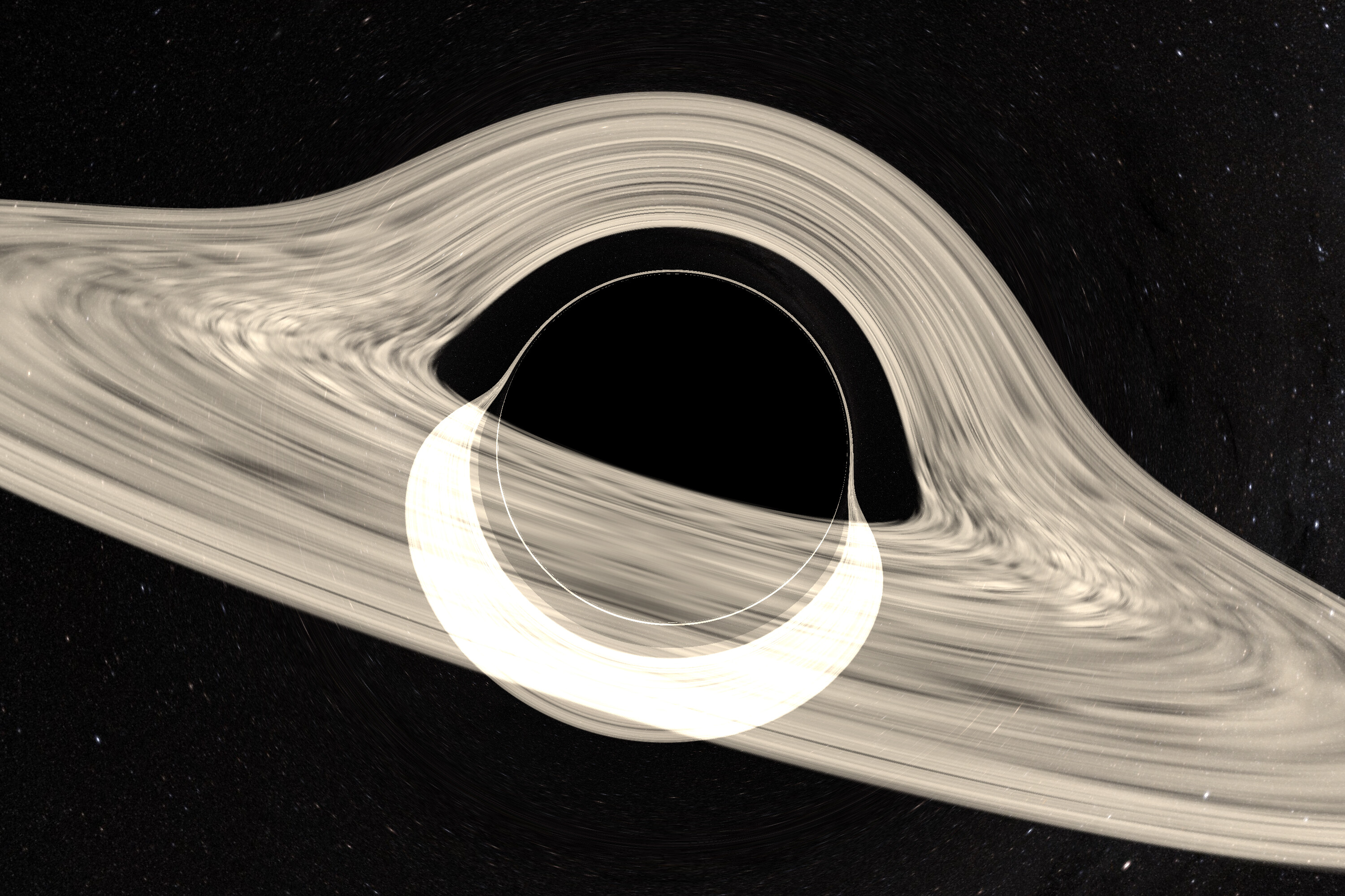
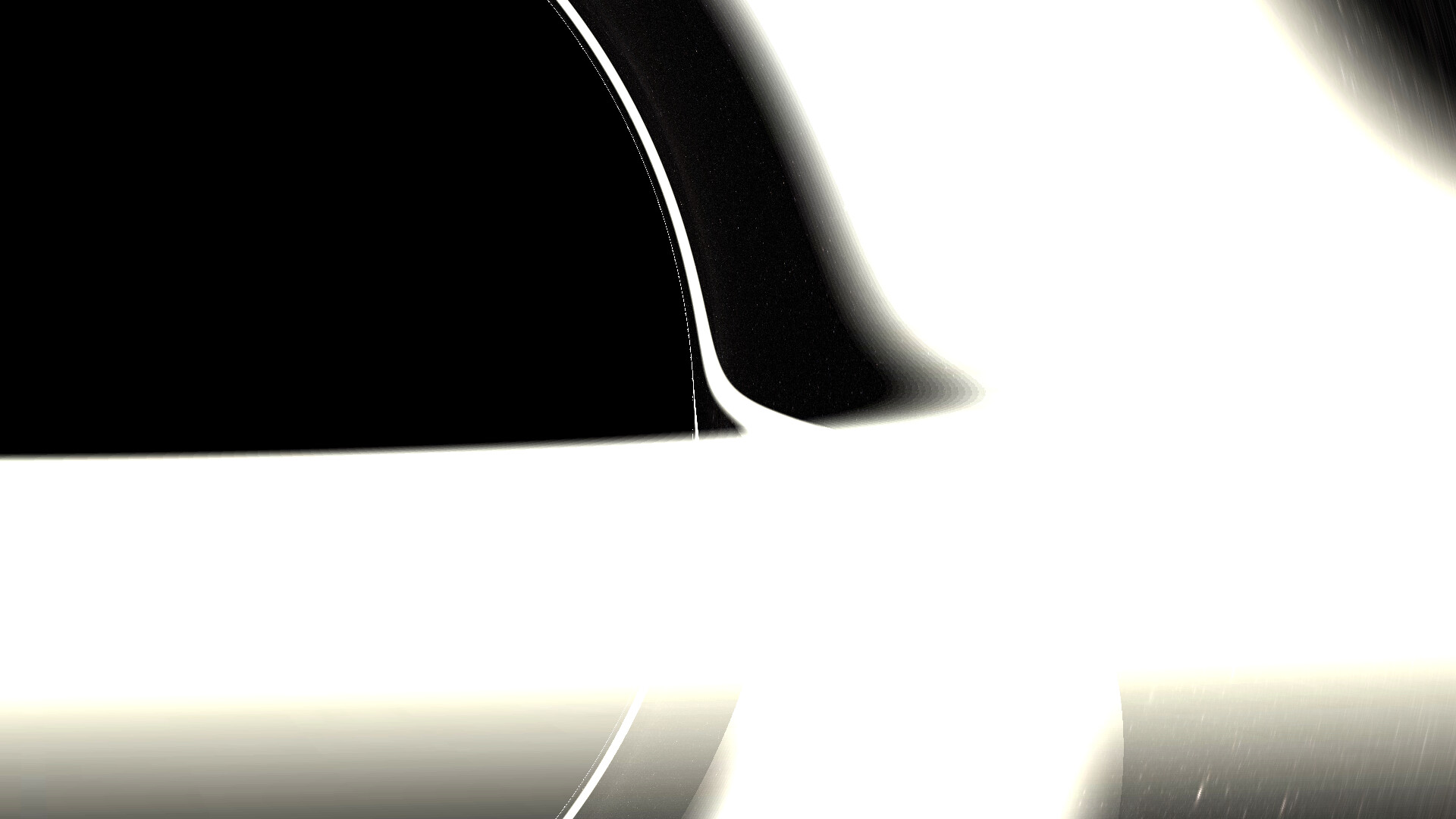
The ray tracer supports an accretion disk that is either textured or plain-colored. It also supports multiple disks, at arbitrary radii from the event horizon, albeit restricted to the horizontal plane around the black hole. The collision point of the ray with the disk is calculated by performing a binary search for the exact intersection. If we don’t search for the precise point of intersection, we would see artifacts due to the “resolution” of the steps taken by each ray (notice the jagged edges at the bottom of the disk):

Once the intersection search is implemented, the lines and borders become nice and crisp:

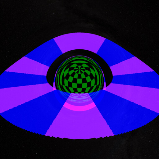
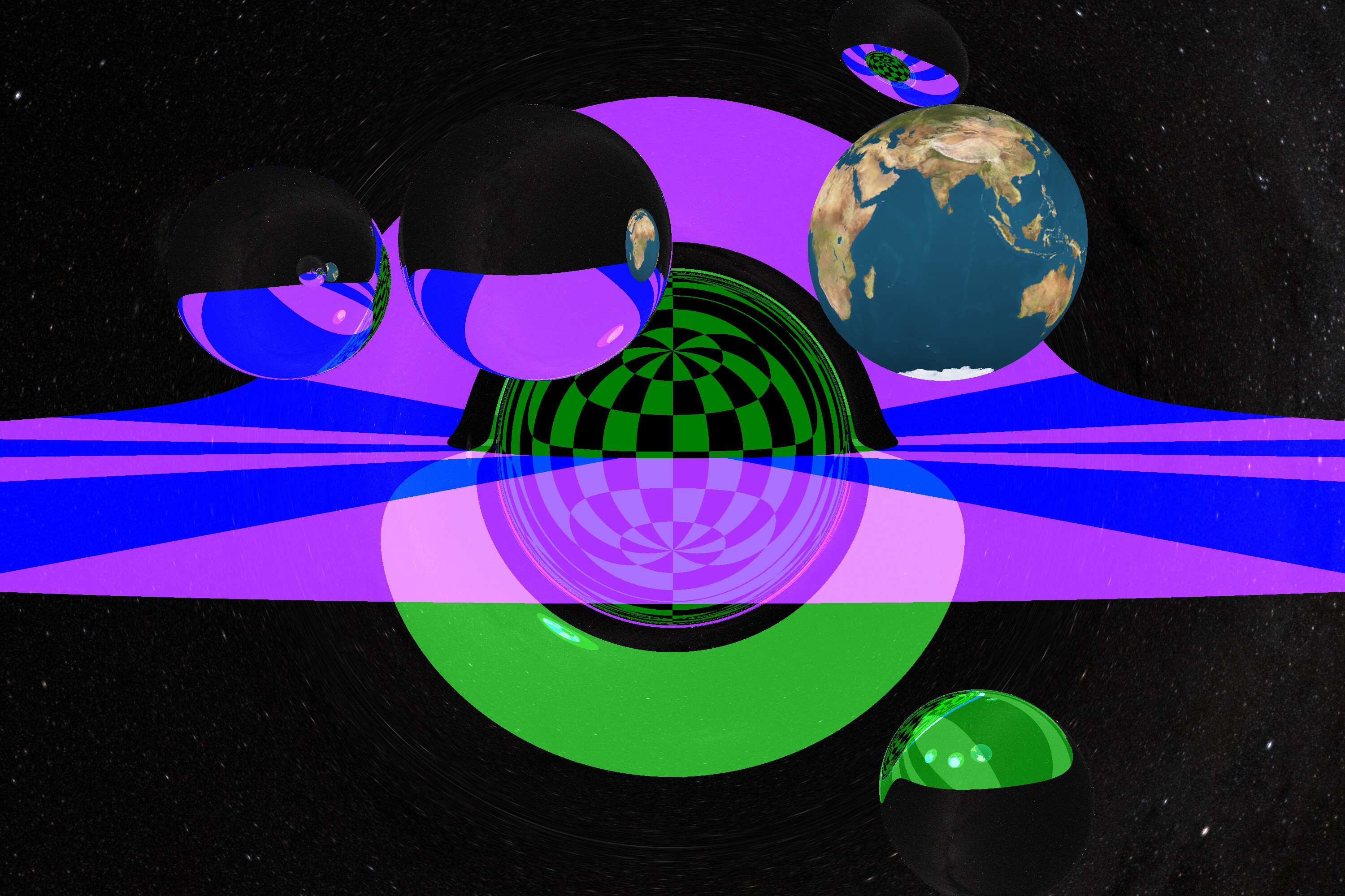
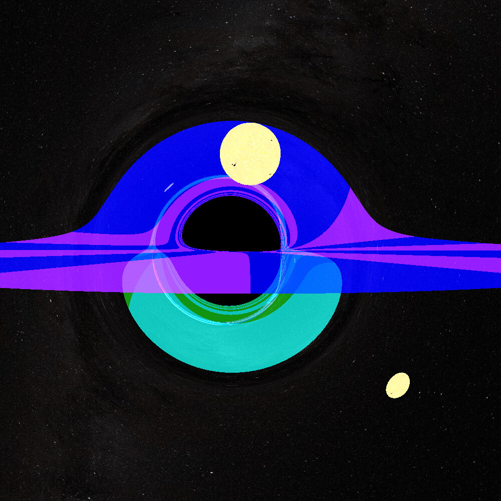
We can also apply different colors to the top and bottom of the disk. Observe that the black hole distorts the disk in a way that makes the bottom (colored in green) appear around the lower semicircle of the photon sphere, even though we’re looking at the disk from above:

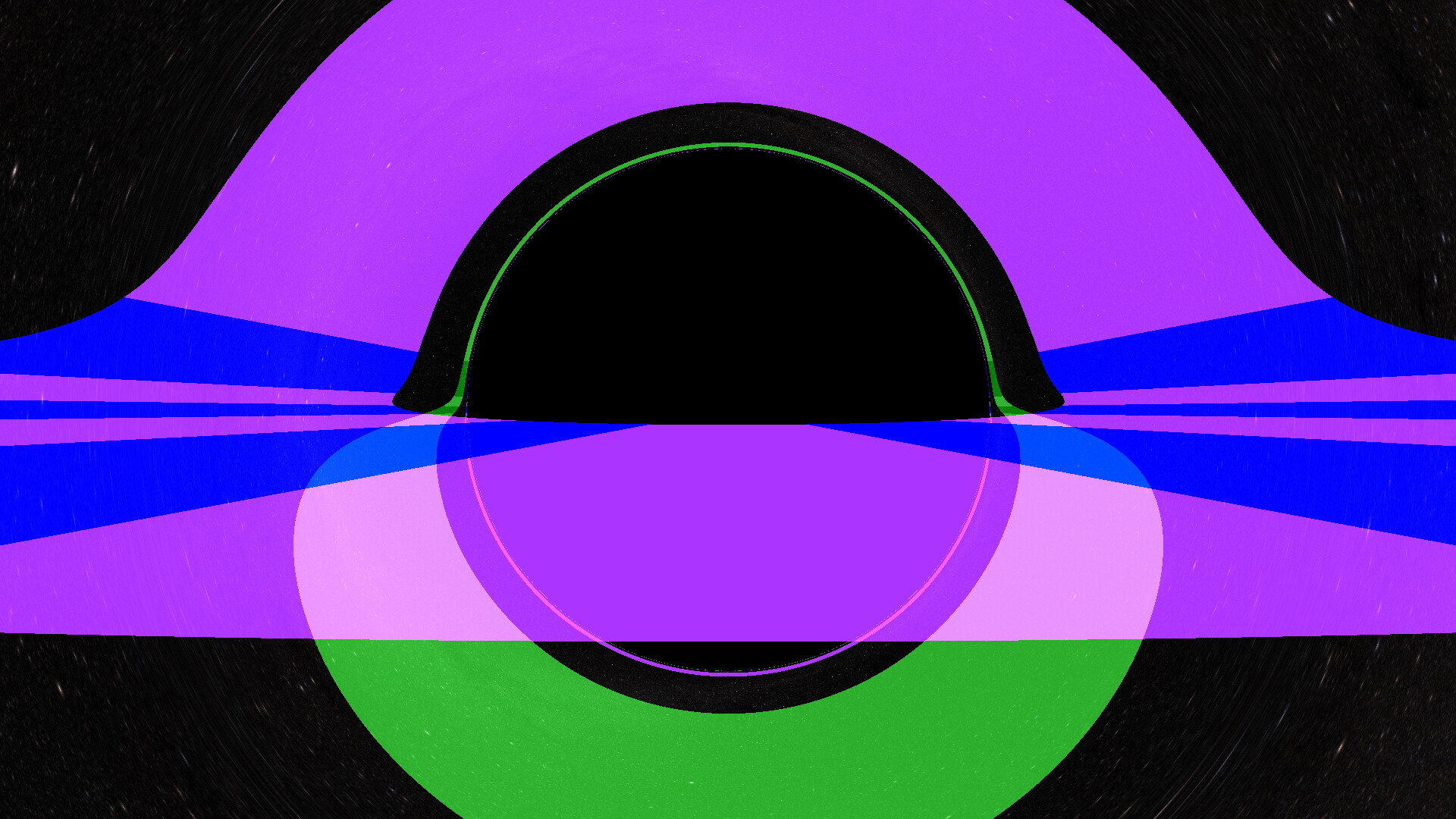
Note that the dark black circle is not the event horizon, but is actually the photon sphere. This is because photons that cross into the photon sphere from the outside cannot escape. (Only photons that are emitted outward from inside the photon sphere can be seen by an outside observer.)

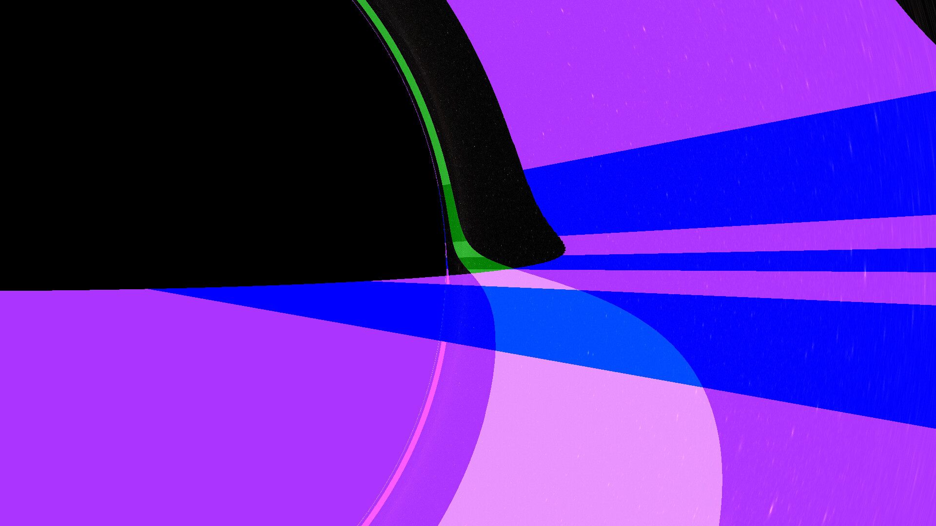
If we zoom in on the right edge of the photon sphere, we can see higher-order images of the disk appear around the sphere (second- and even third-order images are visible). These are rays of light that have circled around the photon sphere one or more times, and eventually escaped back to the observer.

And here is the same image with a more realistic-looking accretion disk:

Great! Now that we have the basics out of the way, it’s time to get a little more crazy with ray tracing arbitrary materials around the black hole.

Additional spheres

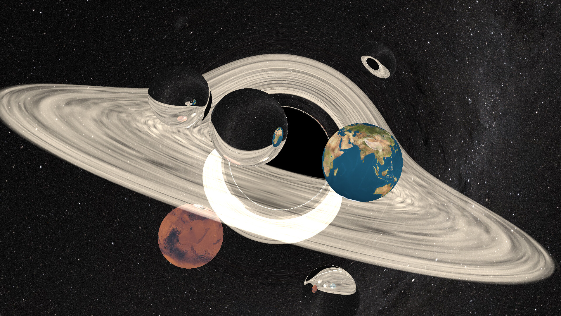
The ray tracer allows adding an unlimited number of spheres, positioned anywhere (outside the event horizon, that is!) and either textured or plain-colored. Here is a scene with one hundred “stars” randomly positioned in an “orbit” around the black hole (click to view larger versions of the images):

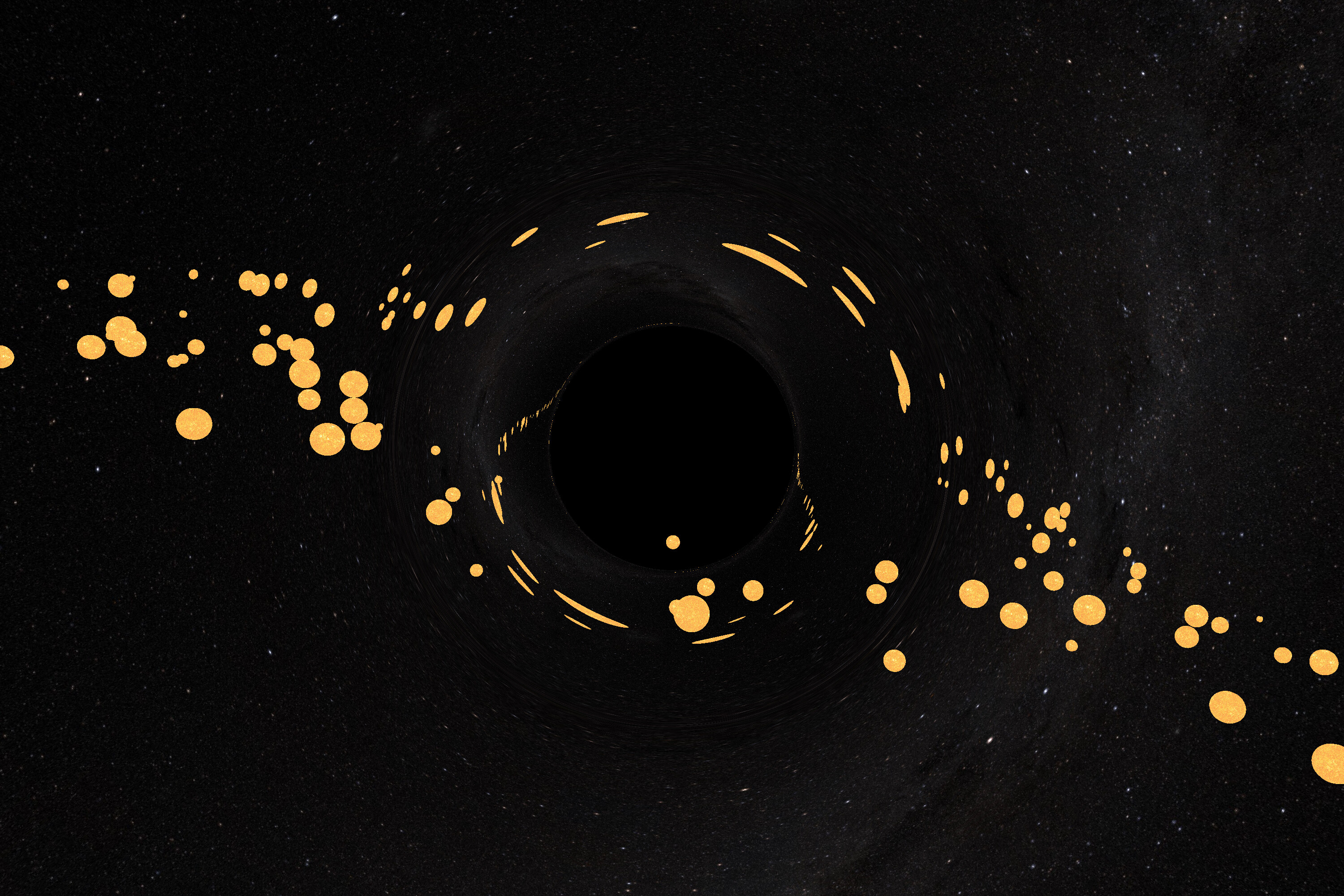
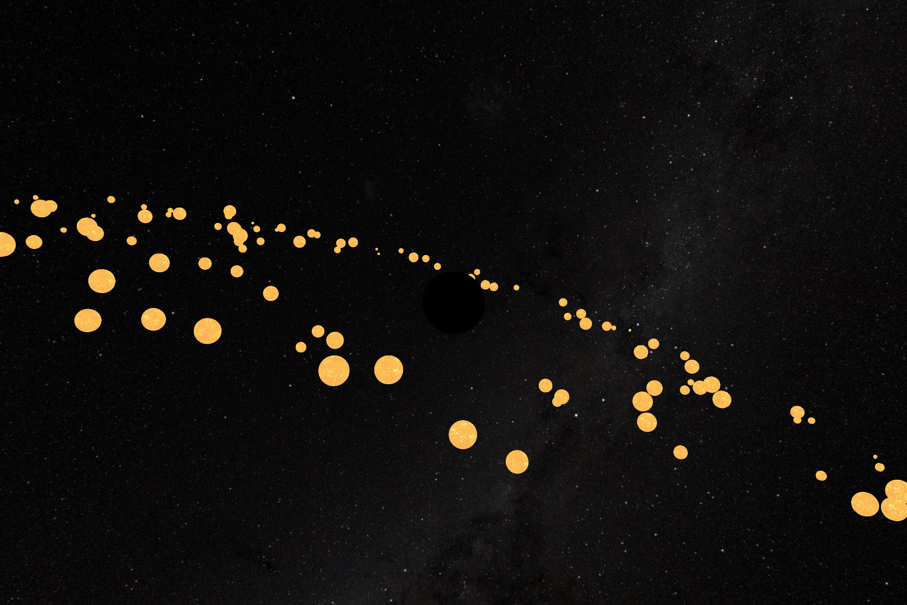
Notice once again how we can see second- and third-order images of the spheres as we get closer to the photon sphere. By the way, here is a similar image of stars around the black hole, but with the curvature effects turned off (as if the black hole did not curve the surrounding space):

And here is a video, generated using the ray tracer, that shows the observer circling around the black hole with stars in its vicinity. Once again, this is not a completely realistic physical picture, since the stars are not really “orbiting” around the black hole, but rather it’s a series of snapshots taken at different angles:

Notice how the spherical stars are distorted around the Einstein ring, as well as how the background sky is affected by the curvature.

Reflective spheres

And finally, the ray tracer supports adding spheres that are perfectly reflective:

All that’s necessary for doing this is to calculate the exact point of impact by the ray on the sphere (again using a binary intersection search) and get the corresponding reflected velocity vector based on the normal vector on the sphere at that point. Here is a similar image, but with a textured accretion disk:

Future work

Eventually I’d like to incorporate more algorithms for different equations of motion for the rays. For example, someone else has encoded a similar algorithm for a Kerr black hole (i.e. a black hole with angular momentum), and there is even a port of it to C# already, which I was able to integrate into my ray tracer easily:

A couple more ideas:

• There’s no reason the ray tracer couldn’t support different types of shapes besides spheres, or even arbitrary mesh models (e.g. STL files).
• I’d also like to use this ray tracer to create some more animations or videos, but that will have to be the subject of a future post.
• Make it run on CUDA?